[This post describes LD prune as implemented in 0.1. The 0.2 version is greatly improved, with a new global pruning strategy based on block-sparse matrix multiplication; see the 0.2 documentation for more details].
Some people have asked about cluster configuration and input parameter settings for LD prune on the Gitter channel. I wrote this post to help answer these questions by giving insight into how LD prune is implemented in Hail.
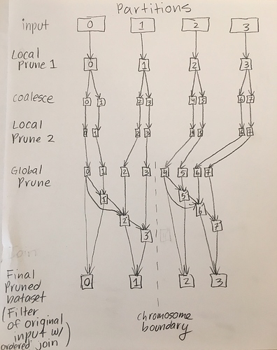
ld_prune() consists of 3 stages. The first two are local prunes where each partition is pruned independently. The last stage is a global prune step where data is shuffled across the network.
The first local prune step does not change the number of partitions besides filtering the variants based on R^2.
After the first prune step, the data is coalesced to N partitions. N is computed by comparing the amount of work that can be done in parallel to optimize the number of cores in the cluster N_optimal = (num_cores * 3) and how many partitions are required for all variants to fit in memory for the entire partition (N_minimum = nVariantsAfterPrune1 / maxNumVariantsPerPartition where maxNumVariantsPerPartition = (memory_per_core * 0.25) / ((8 * nSamples / 32) + 50). Hail will choose to coalesce to the optimal number of partitions if that number is larger than the minimum number needed for all variants to fit in memory (N = if (N_optimal > N_minimum) N_optimal else N_minimum). We found that keeping memory_per_core at the default of 256MB helped prevent out of memory failures.
The second local prune step does not change the number of partitions – it just filters out variants based on R^2.
The last global prune step is an extremely complicated DAG where there is a lot of network shuffling. For example, pruning the second partition is dependent on the variants in the first partition, so we must have the data for both 1 and 2 on the same computer. Partition 3 depends on a pruned version of partition 2 and potentially partition 1 if the window size is big enough that 1MB spans more than 1 partition. You can imagine how this can get complicated very quickly for large datasets.
Unfortunately, there isn’t a one-size fits all answer on what the best input parameters are. You want to take advantage of parallelism for the local prune steps by having more partitions, but you also don’t want too many partitions such that the global prune has a lot of shuffling to do across the network and the dependency trees are extremely complicated. This can cause problems if an executor dies or a task fails and partitions need to be recomputed. However, if the partitions are too big, then you can’t fit all of the data required to prune a partition on a single computer.
